一、比赛简介
1.1 比赛目的
这个kaggle比赛是由Sigma和RentHop两家公司共同推出的比赛。比赛的数据来自于RentHop的租房信息,大概的思路就是根据出租房的一系列特征,比如地理位置(经纬度、街道地址)、发布时间、房间设施(浴室、卧室数量)、描述信息、发布的图片信息、价格等来预测消费者对出租房的喜好程度。
这样可以帮助RentHop公司更好地处理欺诈事件,让房主和中介更加理解租客的需求与偏好,做出更加合理的决策。
1.2 数据集
在这个比赛中,房源的数据来自于renthop网站,这些公寓都位于纽约市。其目的之前已经提到过了,就是基于一系列特征预测公寓房源的受欢迎程度,其目标变量是:interest_level,它是指从在网站上发布房源起始的时间内,房源的询问次数。
其中,比赛一共给了五个数据文件,分别是:
- train.json:训练集
- test.json:测试集
- sample_submission.csv:格式正确的提交示例
- images_sample.zip:租房图片集(只抽取了100个图片集)
- kaggle-renthop.7z:所有的租房图片集,一共有78.5GB的压缩文件。
给出的特征的含义:
- bathrooms: 浴室的数量
- bedrooms: 卧室的数量
- building_id:
- created:发布时间
- description:一些描述
- display_address:展出地址
- features: 公寓的一些特征
- latitude:纬度
- listing_id
- longitude:经度
- manager_id:管理ID
- photos: 租房图片集
- price: 美元
- street_address:街道地址
- interest_level: 目标变量,受欢迎程度. 有三个类: ‘high’, ‘medium’, ‘low’
1.3 提交要求
这个比赛使用的是多分类对数似然损失函数来评价模型。因为每一个房源都有一个对应的最准确的类别,对每一个房源,需要提交它属于每一类的概率值,它的计算公式如下:
其中$N$是测试集中的样本数量,$M$是类别的数量(3类:high、medium、low),$log$是自然对数,$y_{ij}$表示样本$i$属于$j$类则为1,否则为0.$p_{ij}$表示样本$i$属于类别$j$的预测概率值。
一个样本的属于三个类别的预测可能性不需要加和为1,因为已经预先归一化了。为避免对数函数的极端情况,预测概率被替代为$max(min(p,1-10^{-15}),10^{-15})$
最后提交的文件为csv格式,它包含对每一类的预测概率值,行的顺序没有要求,文件必须要有一个表头,看起来像下面的示例:
| listing_id | high | medium | low | |
|---|---|---|---|---|
| 7065104 | 0.07743 | 0.23002 | 0.69254 | |
| 7089035 | 0.0 | 1.0 | 0.0 |
二、Exploratory Data Analysis
在进行建模之前,我们都会对原始数据进行一些可视化探索,以便更快地熟悉数据,更有效进行之后的特征工程和建模。
我们先导入一些EDA过程中所需要的包:
|
|
其中numpy和pandas是数据分析处理中最流行的包,matplotlib和seaborn两个包用来绘制可视化图像,使用%matplotlib命令可以将matplotlib的图表直接嵌入到Notebook之中(%是魔术命令)。
2.1 数据初探
使用pandas打开训练集文件train.json,取前两行观测:
|
|
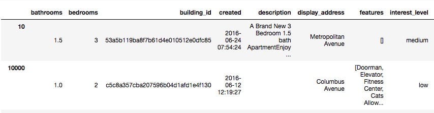
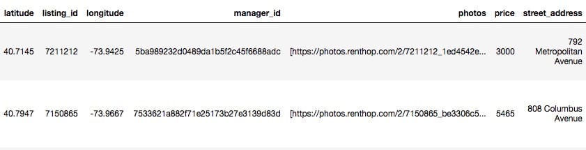
我们可以看到给定的数据中包含各种类型的特征,按照其特征可以分为以下几个类别:
| 特征类型 | 特征 |
|---|---|
| 数值型 | bathrooms、bedrooms、price |
| 高势集类别 | building_id、display_address、manager_id、street_address |
| 时间型 | created |
| 地理位置型特征 | longitude、latitude |
| 文本 | description |
| 稀疏特征 | features |
| id型特征 | listing_id、index |
看一下训练集和测试集分别有多少
|
|
Train Rows: 49352
Test Rows: 74659
训练集有49352个样例,测试集有74659个样例。
接下来我们一一对这些特征进行探索。
2.2 目标变量
在深入探索之前,我们先看看目标变量Interest level
|
|
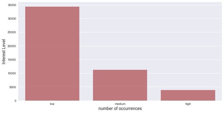
兴趣度在大多数情况下都是低的,其次是中等,只有少部分的样例为高分。
2.3 数值型特征
2.3.1 浴室(bathrooms)
先看看浴室的数量分布
可以看到绝大多数的样例的浴室数量为1,其次为2个浴室。
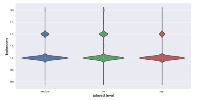
再看看不同兴趣程度的浴室数量分布,运用小提琴图来呈现:
|
|

可以看到在不同的兴趣程度上,浴室数量的分布差不多。
2.3.2 卧室(bedrooms)
|
|
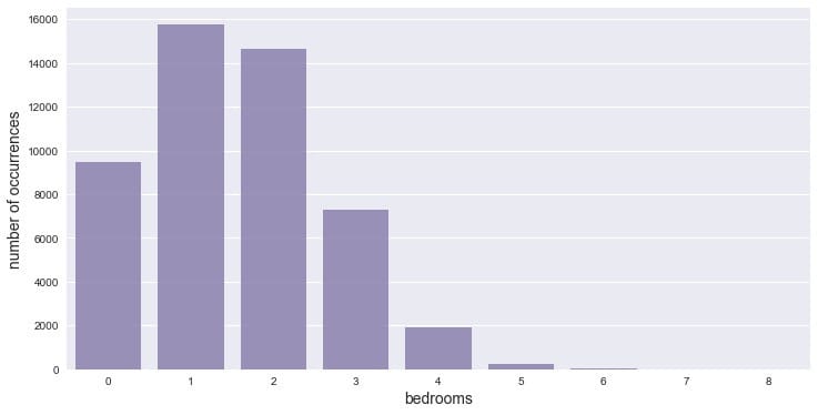
卧室数量基本集中在1和2,也有不少没有卧室,3个卧室的房子也不少。
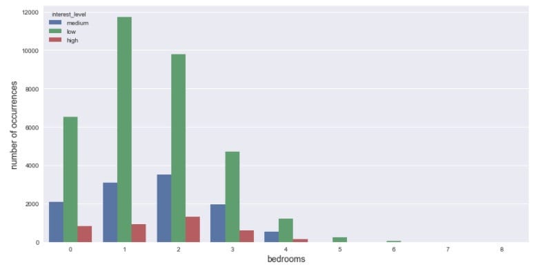
看看不同兴趣程度的卧室数量分布,同样也用小提琴图来呈现:
|
|
2.3.3 价格(price)
对价格排序,看一下价格的分布:
|
|
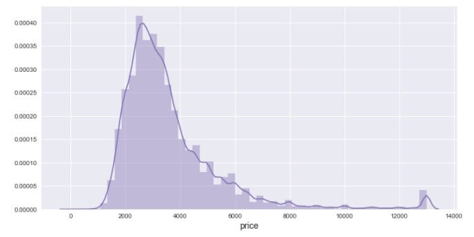
可以观察到有几个价格格外的高,视为异常值,我们把它们移除掉,然后再绘制分布直方图。
|
|

可以观察到分布略微有点右偏。
2.4 地理位置型
2.4.1 纬度(latitude)
先看看纬度的分布情况
|
|
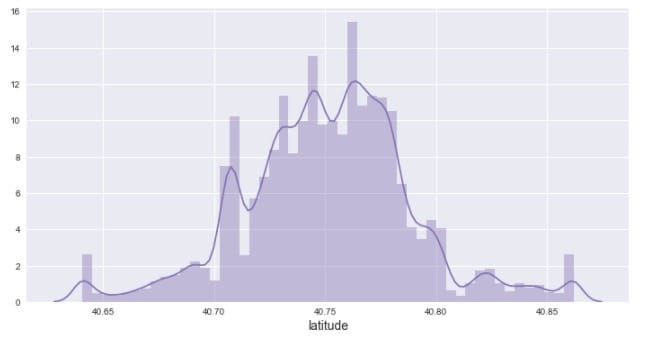
由图可知,纬度基本上介于40.6到40.9之间
2.4.2 经度(longitude)
|
|
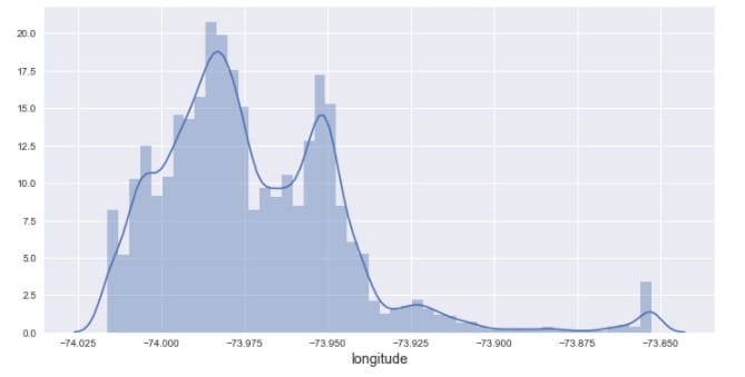
经度介于-73.8和-74.02之间。
接下来,我们尝试把经纬度对应到地图上,绘制成热图,也就是房源在地理位置上的分布密度图。
|
|
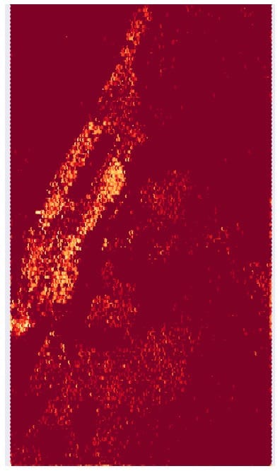
基本和纽约市的城市热图相匹配。
2.5 时间型
2.5.1 发布时间(Created)
先看一下不同时间的分布状况。
|
|
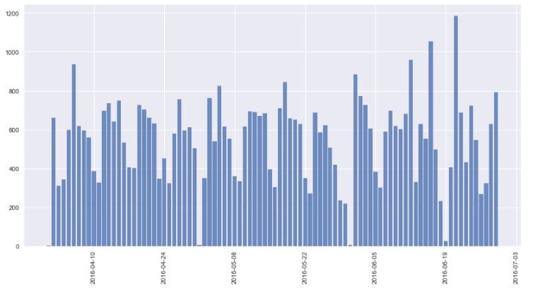
从图中观察到发布时间是从2016年的4月至6月,当然这是训练集的情况,对应的,再看看测试集的发布时间状况。
|
|
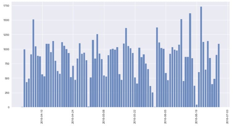
可知,测试集的时间分布和训练集类似。
再看看不同时刻的样本分布情况:
|
|
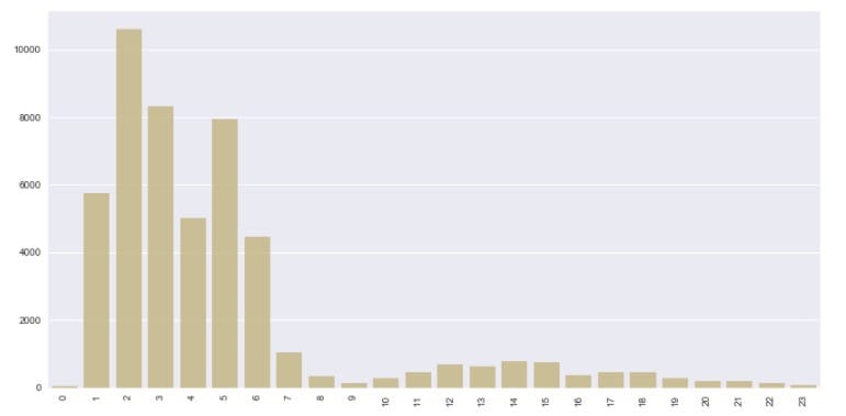
看起来像是一天中比较早的几个小时创建的比较多。可能是那个时候流量不拥挤,数据就更新了。
2.6 其他类型特征
2.6.1 展示地址(Display Address)
|
|
上述代码中(cnt_srs<i)返回的是布尔值True | False。再求一个
得到的结果为:
Display_address that appear less than 2 times:63.22%
Display_address that appear less than 10 times:89.6%
Display_address that appear less than 50 times:97.73%
Display_address that appear less than 100 times:99.26%
Display_address that appear less than 500 times:100.0%
绘制展示地址频次分布直方图:
|
|
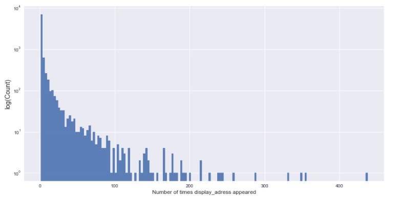
大部分的展览地址出现次数在给定的数据集中少于100次。没有超过500次的。
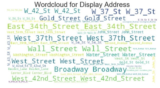
再看看展示地址的词云图:
|
|
2.6.2 照片数量(Photos)
这个比赛也有巨大的照片数据。让我们先看看照片的数量:
|
|
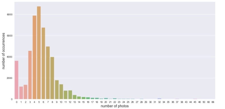
大多数样例的照片数量集中在3~8张。
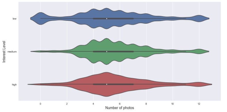
再来看看不同兴趣程度下的照片数量分布:
|
|
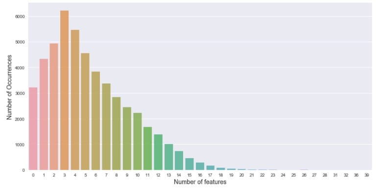
2.6.3 描述特征的数量(features)
每一个房源都对应一个features列,它描述了该样例的特征,比如位于市中心呀、能养猫呀、可以肆意遛狗,类似于这种亲民的特点。有的时候,这种利民条件越多,或许会提高消费者的兴趣,当然也不一定,可以先来看看特征数量的分布:
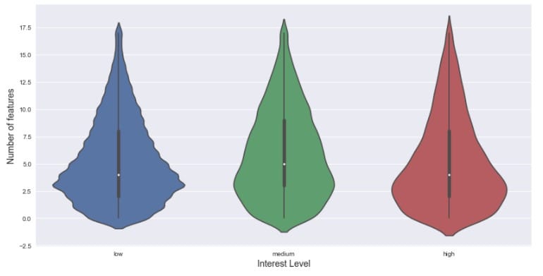
再看看不同兴趣程度下的描述特征数量分布:
|
|
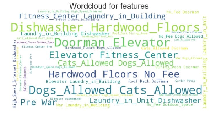
也可以看看描述特征的词云:
|
|
以上这些探索性分析只是对原始数据初步的认识与了解,完了就可以建立一个base model。随着之后的特征工程对其进行更深层次的探索挖掘,不断迭代,使得我们的模型的预测效果越来越好。下一篇就开始着手建立一些base model。

