数据分析系列（4）：基于ARMA模型的资金渠道流入流出预测

该数据为某资金渠道从2017/01/01至2017/07/29这段时间内的清算金额汇总信息，每5分钟按流入流出汇总交易数据，type为SE表示流入，type为RE表示流出，其中2017/01/01至2017/07/23这段时间的每天各时段的流入流出汇总数据是齐全的，而2017/07/24至2017/07/29这六天时间只有0点到早上10点的数据。现在要求我们根据这些数据来预测这六天每天从当日0点到24点的流入流出轧差值（总流入-总流出）。

通过观察我们可以得知这些资金流入流出数据是各时间点上形成的数值序列，而时间序列分析就是通过观察历史数据预测未来的值，适用于我们这次预测。

自回归移动平均模型(ARMA(p，q))是时间序列中最为重要的模型之一，它主要由两部分组成： AR代表p阶自回归过程，MA代表q阶移动平均过程，其公式如下：

$$Z_t=\varphi _1z_{t-1}+\varphi _2z_{t-2 }+···+\varphi _pz_{t-p}+a_t-\theta_1a_{t-1}-···-\theta_qa_{t-q}$$

可以对其简化：

$$\varphi_p(B)z_t=\theta_q(B)a_t\\其中\varphi_p(B)=1-\varphi_1B-\varphi_2B^2-···-\varphi_pB^p\\\theta_q(B)=1-\theta_1B-\theta_2B^2-···-\theta_qB^p$$

一、分析过程

1.1 数据预处理

首先要对数据进行转换处理，type为SE的amount保持不变，type为RE的amount取负数，对缺失值记为0，这样可以方便之后处理，将数据存入字典中，key为时间，value为资金（有正负）。处理脚本如下：

def Data_Process(input_file,header= True):
    amount_dict={}
    for line in open(input_file):
        term = line.strip().split(',')   
        if header:
            header =False
            continue
        if term[1]=='SE': 
            if term[2] =='':
                amount =0
            else:
                amount = float(term[2])
        elif term[1]=='RE':
            if term[2] =='':
                amount =0
            else:
                amount = -1*float(term[2])
        time = datetime.strftime(datetime.strptime(term[0],'%Y/%m/%d %H:%M'),'%Y/%m/%d %H:%M')
        if not time in amount_dict:
            amount_dict[time] = round(amount,2)
        elif time in amount_dict:
            amount_dict[time]+=round(amount,2)
    return  amount_dict

因为我们要对天级别的数据进行预测，可以对资金按天进行聚合：

def dataframe_trans_series(amount_dict,freq='D'):
    data_dict={}
    data_dict['amount'] = amount_dict
    data = pd.DataFrame(data_dict)
    data.index = pd.to_datetime(data.index) 
    df = pd.DataFrame(data['amount'].resample(freq).sum())
    time_series =  df['amount']
    return time_series

得到的中间数据如下所示，每一天对应一条数据，表示这一天的流入流出轧差值：

2017-01-01    123081.02
2017-01-02    150143.02
2017-01-03    161112.42
2017-01-04    138823.62
2017-01-05    130364.32
2017-01-06     85308.56
2017-01-07     77484.16
2017-01-08     93860.22
······

1.2 绘制时序图

按天聚合之后，我们可以简单看一下时序图、移动平均时序图和加权移动平均时序图：

def draw_trend(timeSeries, size):
    f = plt.figure(facecolor='white')
    
    rol_mean = timeSeries.rolling(window=size).mean()
    rol_weighted_mean = pd.ewma(timeSeries, span=size)
    timeSeries.plot(color='blue', label='Original')
    plt.legend(loc='best')
    plt.title('Original')    
    rol_mean.plot(color='red', label='Rolling Mean')
    plt.legend(loc='best')
    plt.title('Rolling Mean')    
    rol_weighted_mean.plot(color='black', label='Weighted Rolling Mean')
    plt.legend(loc='best')
    plt.title('Weighted Rolling Mean')    
    plt.show()

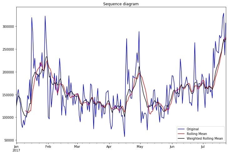
可以从时序图看出，该时间序列存在着波动，尚无法确定是否平稳，需要进一步的统计检验。

1.3 平稳性检验

序列的平稳性是进行时间序列分析的前提条件，单位根检验（ADF）是一种常用的平稳性检验方法，他的原假设为序列具有单位根，即非平稳，对于一个平稳的时序数据，就需要在给定的置信水平上显著，拒绝原假设。

def test_Stationarity(ts):
    test = adfuller(ts)
    output = pd.Series(test[0:4], index=['Test Statistic','p-value','Lags Used','Number of Observations Used'])
    for key,value in test[4].items():
        output['Critical Value (%s)'%key] = value
    return output

以下为检验结果，其p值小于0.01，说明拒绝原假设，得出此序列具有平稳性。

Test Statistic                  -3.779937
p-value                          0.003119
Lags Used                        2.000000
Number of Observations Used    201.000000
Critical Value (5%)             -2.876029
Critical Value (1%)             -3.463309
Critical Value (10%)            -2.574493

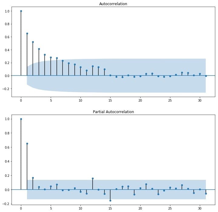
当然也可以观察其自相关图，可以看到，其自相关图快速衰减，体现了平稳性序列的特点，可认为他是平稳序列。

def draw_acf_pacf(ts, lags=31):
    f = plt.figure(figsize=(12,12),facecolor='white')
    ax1 = f.add_subplot(211)
    plot_acf(ts, lags=31, ax=ax1)
    ax2 = f.add_subplot(212)
    plot_pacf(ts, lags=31, ax=ax2)
    plt.show()

1.4 对数处理

对数变换主要是为了减小数据的振动幅度，使其线性规律更加明显。对数变换相当于增加了一个惩罚机制，数据越大其惩罚越大，数据越小惩罚越小。虽然上一步我们验证了序列是平稳的，取对数也可以在该数据集上使用。

def Log_Process(time_series):
    return np.log(time_series+1)

1.5 纯随机性检验

经过平稳性检验之后，我们得到该序列为平稳性序列，接下来对其进行纯随机性检验，只有当时间序列不是一个白噪声即纯随机序列的时候，我们才可以对该序列做进一步的分析：

def test_stochastic(ts):
    p_value = acorr_ljungbox(ts, lags=1)[1] 
    return p_value

得到的p值如下，可知，该序列为非白噪声序列。

6.09097901e-21

1.6 确定ARMA的阶数

由前面的平稳性检验和纯随机性检验可知，该序列为平稳序列且非白噪声序列，我们可以用ARMA(p,q)模型对其建模，这里关键的是p和q的定阶，我们可以通过观察自相关图ACF和偏自相关图PACF来识别，也可以借助AIC、BIC统计量来确定。

1.6.1 BIC识别

以下是根据设定的maxlag，循环对p、q赋值，选出拟合BIC最小的p、q值作为模型的参数，并输出BIC最小的模型：

def choose_better_model(time_series, maxLag=5):
    init_bic = sys.maxint
    init_p = 0
    init_q = 0
    init_properModel = None
    for p in np.arange(maxLag):
        for q in np.arange(maxLag):
            model = ARMA(time_series, order=(p, q))
            try:
                results_ARMA = model.fit(disp=-1, method='css')
            except:
                continue
            bic = results_ARMA.bic
            if bic < init_bic:
                init_p = p
                init_q = q
                init_properModel = results_ARMA
                init_bic = bic
    return init_bic, init_p, init_q, init_properModel

init_bic = 33.0754219416592  init_p = 1  init_q = 1

得到使BIC最小的模型，bic = 33.1，p、q分别为1。

1.6.2 ACF、BCF识别

通过观察自相关图ACF和偏自相关图PACF来识别。观察下图，发现自相关和偏相系数都存在拖尾的特点，并且他们都具有明显的一阶相关性，所以我们设定p=1, q=1。

1.7 拟合ARAM模型

选出BIC最小的模型，对训练集进行拟合。这里添加了一步将对数处理和差分处理还原的操作：

bic, p, q, properModel = choose_better_model(time_series_diff)    
predict_time_series = properModel.predict()
predict_time_series = recover(predict_time_series, time_series_train, best_diff)

1.8 训练集的拟合优度

用拟合好的模型对训练集进行预测，并使用均方根误差对效果进行衡量：

original_time_series = time_series[predict_time_series.index]  
plt.figure(facecolor='white')
predict_time_series.plot(color='blue', label='Predict')
original_time_series.plot(color='red', label='Original')    
RMSE = np.sqrt(sum((predict_time_series-original_time_series)**2)/original_time_series.size)
plt.title('RMSE: %.4f'% RMSE)
plt.show()
print("训练集的RMSE为："+str(RMSE))

训练集预测值和真实值拟合图如下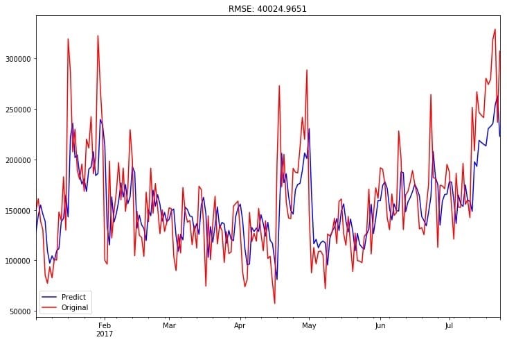：训练集的均方根误差为：

训练集的RMSE为：40024.97

1.9 预测结果

用拟合好的模型对测试集进行预测：

test_predict = properModel.predict(start='2017-07-24', end='2017-07-29')
test_predict = recover(test_predict, time_series_train, best_diff)
print test_predict

得到最终的结果如下：

2017-07-24    244854.689637
2017-07-25    222634.079094
2017-07-26    206351.989143
2017-07-27    194213.093708
2017-07-28    185037.296689
2017-07-29    178024.480144

二、问题

2.1 请给出你的分析过程、预测结果、建模脚本（要求可复现），包含必要的说明以及截图

分析过程和预测结果如上所示，建模脚本见百度网盘，密码：9okf，包括两个文件，一个为jupyter notebook【SERE_PREDICT.ipynb】，一个为python脚本【SERE_PREDICT.py】，两者均可复现。实验环境为python2.7，实验所依赖的package包括：

• pandas
• numpy
• datetime
• matplotlib
• statsmodels

2.2 你认为你的模型预测结果如何，附上关键说明和截图

在本实验中，我使用均方根误差来评价模型预测效果，得到在训练集上的训练集的均方根误差为：40024.97。因为该数据集的数值均较大，日流入流出均达到了十万级别，这样的均方根误差相对来说效果较好，但有较大的提升空间。在分析过程中已有具体的呈现和说明。

2.3 如果需要提高预测准确率，可以从哪些方面入手，简单列举即可

1. 在时间序列中存在的噪声，会干扰序列中每个点的波动，给预测造成难度，可以使用卡尔曼滤波来过滤这个噪声。将卡尔曼滤波算法与ARMA模型结合时，卡尔曼滤波算法可以在当获得一个新的数据点时，递归地更新状态变量（预测值）的信息，可以起到对ARMA模型的修正作用，在一定程度上提高ARMA模型的预测精度。

2. 注意到我们需要预测的那几天在0点至10点是存在资金流动数据的，我们可以将这一部分数据作为我们预测全天数据的先验信息，提高预测精度。

3. 如果我们具有有关资金流动的其他信息，诸如资金流动的来源、股市波动信息、宏观政策的变动、市场波动的信息等等，就可以构建一个特征集，用LSTM（长短时循环神经网络）来对序列进行建模。当然要是没有这些信息，也可以直接用历史记录 $[y_{t-1}, y_{t-2},…]$ 以及他们的各种统计量如均值、最大最小值、一阶差分、二阶差分等对 $x_t$ 做特征工程，以此丰富其维度，再使用LSTM对其进行建模。